Neural networks have minima at infinity. How do they look like?

Consider two neurons in a hidden layer of a standard MLP, with output weights \(a_i, a_j\) and input weight vectors \(\mathbf{w}_i, \mathbf{w}_j\).
Their combined contribution to the network output is: \(y = a_i \ \sigma(\mathbf{w}_i \cdot \mathbf{x}) + a_j \ \sigma(\mathbf{w}_j \cdot \mathbf{x}).\)

Now imagine these two neurons get closer and closer in input space, i.e. their weight vectors nearly coincide, while their output weights blow up in opposite directions: \(a_i - a_j \rightarrow \pm \infty\).

We can make this precise by writing \(\mathbf{w}_i = \mathbf{w} + \epsilon \boldsymbol{\Delta}\) and \(\mathbf{w}_j = \mathbf{w} - \epsilon \boldsymbol{\Delta}\), with \(c = a_i + a_j\) and \(a = \epsilon(a_i - a_j)\) held fixed as \(\epsilon \to 0\). The sum of the two neurons becomes a central finite difference, and in the limit you get

\[a_i \ \sigma(\mathbf{w}_i \cdot \mathbf{x}) \;+\; a_j \ \sigma(\mathbf{w}_j \cdot \mathbf{x}) \;\xrightarrow{\;\epsilon \to 0\;}\; c\,\sigma(\mathbf{w} \cdot \mathbf{x}) \;+\; a\,(\boldsymbol{\Delta} \cdot \mathbf{x})\,\sigma'(\mathbf{w} \cdot \mathbf{x}).\]

The first term is a standard neuron. The second is a gated linear unit: a linear function \(\boldsymbol{\Delta} \cdot \mathbf{x}\) multiplied by the gate \(\sigma'(\mathbf{w} \cdot \mathbf{x})\).
In the demo above you can play with this yourself for a 2D input. Use the sliders to change \(a\) and \(c\), and rotate the orientations of \(\mathbf{w}\) and the pair \(\mathbf{w}_i, \mathbf{w}_j\). In approximation mode, watch the surface morph from a sum of two regular neurons into a gated linear unit as \(\epsilon\) shrinks to zero.

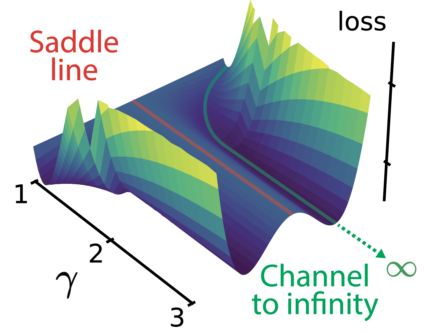
Two standard MLP neurons, can get trapped into a zone of the landscape that makes them drift to infinity, named channel to infinity, spontaneously learning a computational primitive they were never explicitly given. In our NeurIPS 2025 paper Flat Channels to Infinity in Neural Loss Landscapes we find that these solutions happen surprisingly often in regression settings.

Interestingly, these channels to infinity are located parallel to manifolds of saddle points that were first described by Fukumizu & Amari, 2000.

Below a picture of an actual loss landscape, the saddle line in red and the channel to infinity in green.